MDA Overdrive
Simple soft distortion plug-in.
This article is part of the Plug-in Archeology series where we dig through the source code of old plug-ins to figure out how they work.
In this episode we’ll take a look at MDA Overdrive, one of the simpler plug-ins from the MDA suite, making it an ideal starting point for someone who is new to audio development.
I recommend that you grab the code, run it, and try to figure out for yourself first how this plug-in works, and then come back to this article. Reading other people’s source code is a great exercise!
NOTE: The original version of this plug-in was written for VST2 but I ported it to JUCE and modernized it a little. The code shown in this article is modified slightly from the GitHub version, to make it easier to explain how it works.
About the plug-in
MDA Overdrive is a soft distortion plug-in. As the original docs used to say:
Possible uses include adding body to drum loops, fuzz guitar, and that ‘standing outside a nightclub’ sound. This plug does not simulate valve distortion, and any attempt to process organ sounds through it will be extremely unrewarding!
MDA Overdrive does three things to the sound: first it distorts it, then it applies a low-pass filter, and finally it applies output gain.
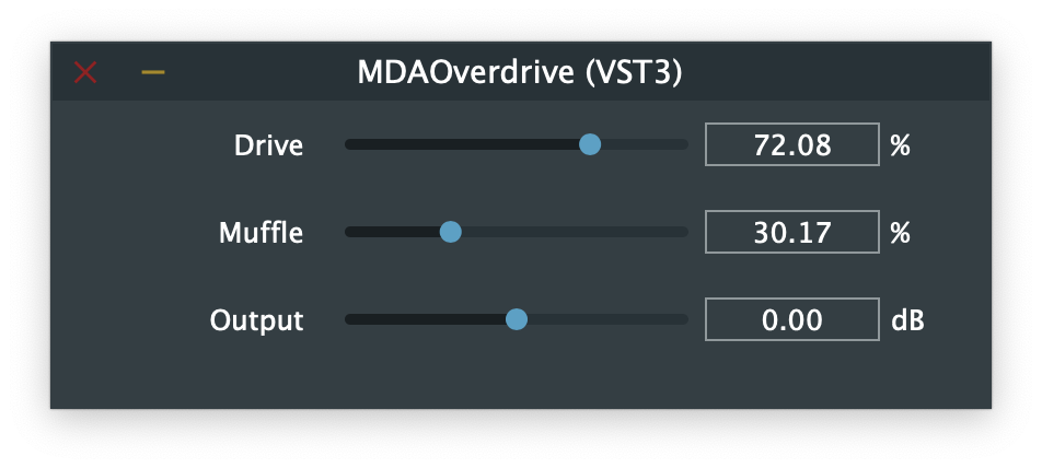
The plug-in has the following parameters:
- Drive: amount of distortion, 0 – 100%
- Muffle: gentle low-pass filter, 0 – 100%
- Output: level trim, –20 dB to +20 dB
These parameters are defined in PluginProcessor.cpp in the createParameterLayout() method and are JUCE AudioParameterFloat objects.
The audio processing loop
The audio processing code for MDA Overdrive is as follows. As is typical for a JUCE plug-in, this happens in the processBlock() method in PluginProcessor.cpp.
for (int i = 0; i < buffer.getNumSamples(); ++i) {
    float a = in1[i];
    float b = in2[i];

    float aa = (a > 0.0f) ? std::sqrt(a) : -std::sqrt(-a);
    float bb = (b > 0.0f) ? std::sqrt(b) : -std::sqrt(-b);

    float xa = drive * (aa - a) + a;
    float xb = drive * (bb - b) + b;

    fa = fa + filt * (xa - fa);
    fb = fb + filt * (xb - fb);

    out1[i] = fa * gain;
    out2[i] = fb * gain;
}
That’s the whole thing! Looks simple enough, but if you’re new to audio programming it may not immediately make sense what’s going on here. Don’t worry, I’ll go over each line and explain what it does.
The variables in1 and in2 are float* pointers to the input audio buffer for the left and right channel, respectively, while out1 and out2 are pointers to the output buffers. In JUCE, these pointers are obtained like so:
const float* in1 = buffer.getReadPointer(0);
const float* in2 = buffer.getReadPointer(1);
float* out1 = buffer.getWritePointer(0);
float* out2 = buffer.getWritePointer(1);
To keep thing simple, this plug-in assumes it’s being used on a stereo track, so there are always two channels. It wouldn’t be too hard to change the plug-in to also support mono. In JUCE this can be done by modifying the isBusesLayoutSupported() method.
Applying gain
Let’s now look at each line of the audio processing logic in detail, beginning with the output gain. Here is the loop again:
for (int i = 0; i < buffer.getNumSamples(); ++i) {
    float a = in1[i];
    float b = in2[i];

    /* do the audio processing */

    out1[i] = fa * gain;
    out2[i] = fb * gain;
}
This steps through each sample in the current audio buffer and reads the sample value for the left channel into variable a and the sample value for the right channel into b.
I’m using the variable names from the original code here, which perhaps are a bit on the short side, but in small code snippets such as this I don’t mind using short variable names.
After reading the input samples, we do the actual audio processing. This puts the results into two new variables, fa and fb. Before these values are placed into the output audio buffer, they are first multiplied by gain.
The gain variable corresponds to the plug-in’s Output parameter, which is given in dB or decibels. The following code converts the amount in decibels to a number between 0 and 1.
float output = apvts.getRawParameterValue("Output")->load();
gain = juce::Decibels::decibelsToGain(output);
This code lives in a method named update() that is called from processBlock() before the audio processing loop, so that every time the plug-in has to render a new block of audio we first read the parameter values.
Two things of note here:
-
Using
getRawParameterValue()isn’t very efficient, as it performs relatively slow string comparisons to look up the parameter name. It would be better to create a pointer to theAudioParameterFloatvariable that represents this parameter and use that directly. However,getRawParameterValue()is good enough for a simple example like this. -
There is no parameter smoothing in this plug-in. If you move the Output slider rapidly back-and-forth, you’ll hear so-called zipper noise. The MDA plug-ins did not incorporate any parameter smoothing, but feel free to add this yourself, for example using JUCE’s
LinearSmoothedValueclass.
OK, I’m sure you’ve seen how to implement gain in a plug-in before, so let’s look at the more interesting lines from the audio processing code.
Creating distortion
There are many ways to create distortion but it always involves some kind of nonlinear processing. This is also known as waveshaping.
MDA Overdrive uses the absolute square root function:
float aa = (a > 0.0f) ? std::sqrt(a) : -std::sqrt(-a);
float bb = (b > 0.0f) ? std::sqrt(b) : -std::sqrt(-b);
Here aa is the distorted value for the left channel and bb for the right channel.
How this works: If you take a common sine wave — the most elementary waveform that we work with in audio — and apply the above formula to it, you get something that looks like the following:
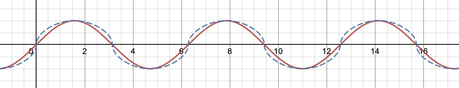
The red curve is the original sine wave, the blue curve is the distorted version. Note how everything is made a little rounder, that’s what creates the distortion. It adds additional frequencies or harmonics to the sound. This will also make everything a bit louder, which is why there is a parameter to change the output level.
The reason the code does -std::sqrt(-a) if the sample value is less than zero, is that taking the square root from a negative number is not possible (we don’t want to deal with imaginary numbers here). To avoid that, this first pretends that a is positive so it can take the square root, and then negates the result to make the sample less than zero again.
We want the user to be able to control the amount of distortion, and that’s what the Drive parameter is for. This is a percentage from 0% – 100%. The following code in the update() method sets the drive variable to a value between 0.0 and 1.0:
drive = apvts.getRawParameterValue("Drive")->load() / 100.0f;
Actually applying the distortion to the current sample is done like so:
float xa = drive * (aa - a) + a;
float xb = drive * (bb - b) + b;
What happens here is a linear interpolation between the original sample values from the left and right input buffers (a and b) and their fully distorted versions (from aa and bb respectively). The amount of interpolation is given by drive.
If you’re having trouble seeing that this indeed does a linear interpolation, it’s possible to write out this equation as:
xa = drive * aa - drive * a + a
   = drive * aa + (1 - drive) * a
This mixes a and aa together based on the value of drive. The larger drive is, the more we add the overdriven signal into the mix:
- If you set
driveto 0, thenxa = a. - While if
driveis 1, thenxa = aa. - Any values of
drivein between 0 and 1 give a blend betweenaandaa.
Using sqrt in this way adds odd harmonics to the sound. For example, if you pass a pure 100 Hz sine wave through this plug-in, the distortion section creates additional frequencies at 300 Hz, 500 Hz, 700 Hz, and so on. The larger drive is, the stronger the frequencies of these harmonics will be, and the louder the total sound becomes.
NOTE: You may have noticed we use the exact same code for both the left and right channels, just with different variables. This is typical for audio code that works in stereo, although for plug-ins where both channels are totally independent of each other (like this one), it’s also possible to first process the entire left channel, and then process the entire right channel. This can be done in a second loop, so that you only have to write the audio processing code once.
Filtering the sound
After distorting the sound, it is optionally low-pass filtered if the Muffle parameter is greater than 0%.
The code for this is:
fa = fa + filt * (xa - fa);
fb = fb + filt * (xb - fb);
We need two filters because there are two channels: the first line of code is for the left channel, the second line is for the right channel. A common beginner mistake is to share a single filter between both channels, but this will give very undesirable results.
The filter is a simple exponentially weighted moving average filter, in audio circles better known as a one-pole filter. The difference equation is:
$$ y[n] = \text{filt} * x[n] + (1 - \text{filt}) * y[n - 1] $$
The code implements the same equation, but written slightly differently to perform only a single multiplication instead of two. Mathematically both formulations are equivalent. This again is kind of a linear interpolation, but this time between the new sample $x[n]$, and the previous sample, $y[n - 1]$.
In the code, the variable xa is used as the $x[n]$ for the left channel, and xb is for the right channel. Likewise, fa is the previous output value $y[n - 1]$ from the left channel and fb is the previous output value on the right.
filt is the filter coeffient and determines where the filter’s cutoff point lies. When the Muffle parameter is 0%, filt = 1.0, and the filter is disabled as that makes (1 - filt) equal to 0. As you move the Muffle slider to the right, filt becomes smaller and more smoothing is applied, making the filter cutoff lower.
So how do we set filt? The code in update() is as follows:
float muffle = apvts.getRawParameterValue("Muffle")->load();
filt = std::pow(10.0f, -1.6f * muffle / 100.0f);
This may require some explanation…
Even though Muffle is shown as a percentage to the user, here it’s turned into a value between 1.0 and 0.025 that drops off exponentially. As mentioned before, 1.0 means the filter is disabled. The smaller the value of filt, the lower the filter’s cutoff frequency will be. At 100% or 0.025, the cutoff is around 180 Hz somewhere.
The curve used by the calculation looks like this:
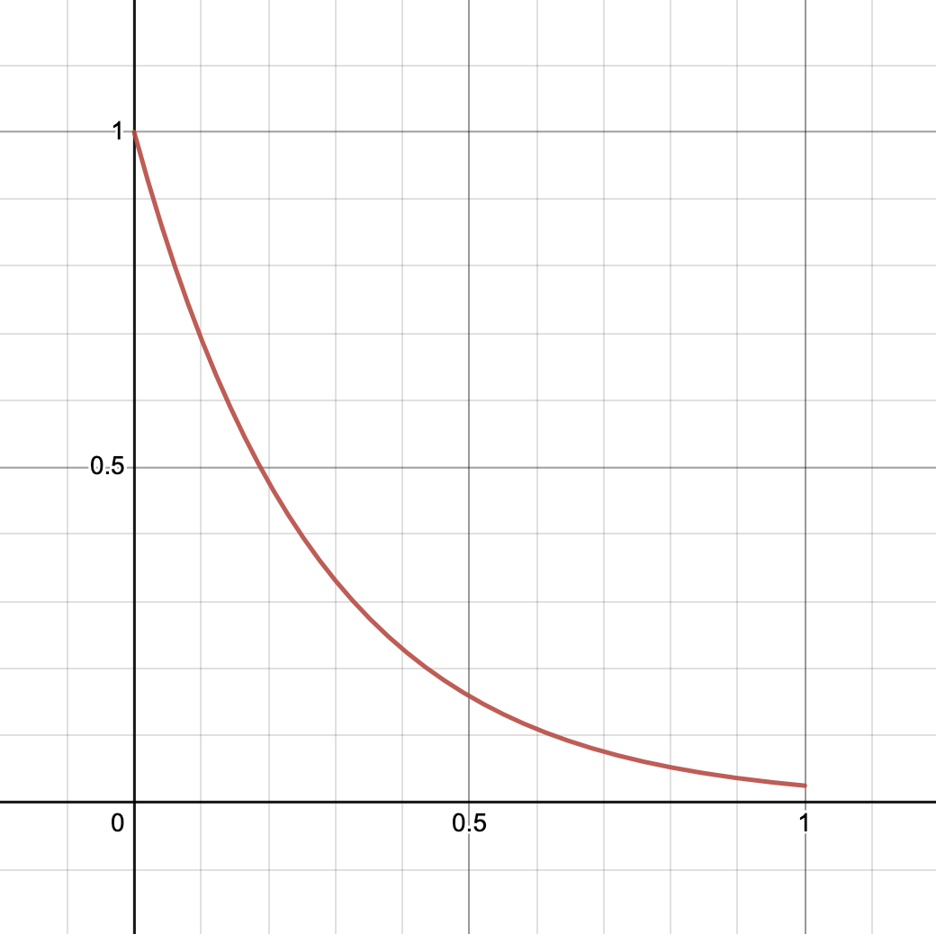
The reason for using this kind of curve is that our perception of frequencies is logarithmic, and so lowering the cutoff point in an exponential manner makes it sound more natural to us than doing it linearly.
The following table shows the difference between a parameter that would work linearly, and a logarithmic one. The closer you move Muffle to 100%, the smaller steps it takes. This is important because differences in low frequencies are more important to human hearing than differences in high frequencies, and so we want more control on the low end.
| Linear parameter | Logarithmic |
|---|---|
| 0% = 22050 Hz | 0% = 22050 Hz |
| 25% = 16538 Hz | 25% = 3600 Hz |
| 50% = 11025 Hz | 50% = 1200 Hz |
| 75% = 5512 Hz | 75% = 450 Hz |
| 100% = 0 Hz | 100% = 180 Hz |
Note that the above formula uses std::pow(10.0f, ...) which is $10^x$, but it also could have used another exponential function such as $2^x$ or $e^x$. The choice is often made fairly arbitrarily, or based on taste and “what feels good”. In the end, all exponential functions can be written in terms of $e^x$ or std::exp() anyway.
The filter cutoff
So how does this filt coefficient actually relate to the filter’s cut-off frequency?
You’ve seen that filt = 1 means no filtering happens, so effectively that puts the cutoff point at or beyond Nyquist (the maximum frequency that can represented by a sampled signal, which is half the sample rate). Technically speaking, for this filter filt = 1 puts the cutoff point infinitely high.
When filt = 0, the cutoff point is at the other end of the spectrum, at 0 Hz, and all sound is completely filtered out. That’s not very useful, which is why filt cannot become smaller than 0.025 in this plug-in.
But how did I know this corresponds to a cutoff point of roughly 180 Hz? Well, I cheated and looked at a spectrum analyzer, but we can also calculate exactly what the cutoff is.
Time for some math! The formula for calculating the filter coefficient of a one-pole filter, when given a certain cutoff frequency, is as follows:
$$ \text{filt} = 1 - \exp(-2 \pi \cdot \text{freq} / \text{sampleRate}) $$
However, we already have filt and want to know freq. To get rid of the exponential, we can use the standard math trick of taking the logarithm of both sides of the equation. After some rewriting, we end up with:
$$ \text{freq} = \frac{-\text{sampleRate} \cdot \log(1 - \text{filt})}{2 \pi} $$
Filling in 44100 for the sample rate and 0.025 for filt gives… 178 Hz. Pretty close.
NOTE: In this formula log means the natural logarithm, which is sometimes written as ln instead. If you are using a calculator to verify this result, make sure you’re using the correct logarithm function or the outcome will not match.
Below, I’ve plotted the possible cutoff frequencies on the vertical axis, versus the Muffle percentage on the horizonal axis. This is clearly an exponential shape, where the range 20% – 100% produces cutoffs below 5 kHz, and percentages lower than 20% give higher cutoffs. Close to 0% the cutoff frequency exceeds Nyquist, which is fine for a simple filter like this.
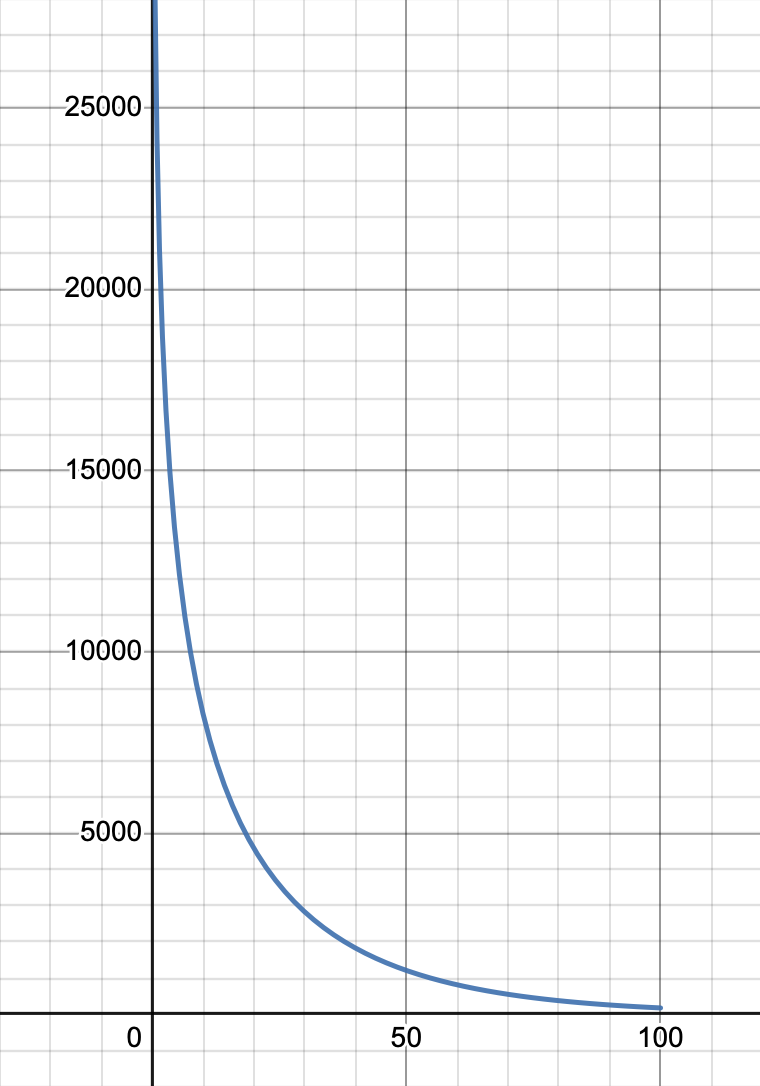
You may also wonder what happens when the sample rate is not 44.1 kHz, but for example 48 kHz. Well, in that case the cutoff point actually lies elsewhere (193 Hz) and the filtering will sound slightly different!
This highlights a problem with the way MDA Overdrive calculates the filter coefficient: it is not independent of the sampling rate. This is typical for older plug-ins, as higher sample rates were not commonly in use back then.
If you’re feeling that all this is rather complicated, I agree. In JUCE you can achieve the same effect by giving the parameter a range in Hz and setting a skew value, and then you don’t have to worry about any of this math. However, if you want a parameter that is expressed as a percentage, then you do need to resort to doing these kinds of calculations yourself.
Denormals
My JUCE implementation of this plug-in also has the following code at the end:
if (std::abs(fa) > 1.0e-10f) filtL = fa; else filtL = 0.0f;
if (std::abs(fb) > 1.0e-10f) filtR = fb; else filtR = 0.0f;
The variables that keep track of the filter state fa and fb are local, so it’s important that we store their values into member variables (filtL and filtR) so they can be used the next time processBlock() is called. Lifting member variables into locals is a practice you’ll see in older code, but is less necessary with modern C++ compilers.
The check for > 1.0e-10f is used to avoid denormal numbers, which are floating-point values that become very small. Denormals are slow as they are handled in software rather than hardware, and for audio they serve no purpose. So when fa or fb become very small, we round them down to zero instead.
In JUCE we don’t need to do this, since the ScopedNoDenormals object that gets created at the top of processBlock() already automatically handles this for us. However, I kept this code since it was part of the original plug-in.
Conclusions
MDA Overdrive is pretty simple but it does show three common techniques that you’ll find in many plug-ins:
- using waveshaping to add harmonical distortion
- using a basic one-pole filter
- applying output gain
One-pole filters appear in lots of places in audio code but, to be honest, they do not make for a great low-pass filter in general. It works fine on the low-end, but the closer the cutoff point is set to Nyquist, the less well the filter responds — it just doesn’t do much at higher frequencies. This is probably also why MDA Overdrive calls the filter parameter “Muffle”, to indicate it works best on low frequencies.
The waveshaper offers only one type of distortion but there are many other nonlinear functions that could be used here. One problem you should be aware of when using waveshaping is that this introduces not only harmonics, which we want, but also aliases, which we don’t want.
An alias is a frequency that exceeds the maximum frequency that can be represented by the sampling rate (the Nyquist limit), and manifests as a lower frequency that adds unwanted buzzing to the sound. One way to deal with the aliasing from waveshaping is to use oversampling, so that the Nyquist limit ends up being higher and the aliases are less important.