FFT Processing in JUCE

A common question that comes up is how to do FFT processing on real-time audio. It’s not as daunting as it may seem but there are some pitfalls to avoid.

The goal here is to periodically apply the Fast Fourier Transform (FFT) to a short fragment of audio to get the frequency spectrum at that point in time, then change this spectrum in some interesting way, and finally use the IFFT (inverse FFT) to turn the modified spectrum back into audio.

This process is known as the Short-Time Fourier Transform or STFT. We use the forward FFT to analyze the audio, and the inverse FFT to resynthesize the audio.

This blog post demonstrates how to do that kind of FFT processing in JUCE. I hope you find it useful!

The example project

The example JUCE project is at: github.com/hollance/fft-juce

The project only has two classes:

• FFTExampleAudioProcessor — the main plug-in object
• FFTProcessor — where all the fun stuff happens

If you’re in a hurry and don’t want to read the rest of this article, simply add your own FFT processing code into FFTProcessor’s processSpectrum() method and you’re ready to rock (but really do read on!).

This is the simplest example I could come up with to demonstrate the STFT technique in a real-time audio context. The code is optimized for readability, not speed.

Read on to learn how the code works and why it does what it does.

You need a FIFO

A fundamental property of the FFT is that it requires a buffer of input samples with a length that is a power of two. A typical size for this buffer is 1024 samples, which gives a spectrum of 1024 frequency bins.

We are going to chop the input audio stream into FFT frames that are each 1024 samples in length, and apply the FFT on each frame:

However, the plug-in will receive audio buffers that can be smaller than 1024 samples and whose length is not necessarily a power of two. Before you can do any FFT processing, you’ll first need to collect enough samples to fill up the next FFT frame.

Collecting samples is typically done using a circular buffer, also known as a “first-in first-out” queue or simply FIFO. This is easier than you might think: a FIFO is just a std::array and a variable that holds a read/write index. This index wraps back to zero when it reaches the end of the array, which is why we call it circular.

The FIFO contains the input samples for a single FFT frame, and is therefore also 1024 elements long. Once we’re done processing the current frame, the read/write index wraps back to the beginning of the FIFO and we’ll simply overwrite the previous contents of the FIFO to fill up the next frame, and so on…

On the output side you also need to use a FIFO. Let’s say we’ve collected our first 1024 samples into the input FIFO and have done our FFT processing on it. Now we have 1024 output samples that need to be played back one at a time over the next 1024 timesteps, which requires a FIFO of its own.

Since we need to wait 1024 timesteps before we have enough samples to perform the next FFT, the output is delayed, also by 1024 timesteps. In other words, the plug-in will have a latency of 1024 samples.

For the input sample at time t and an FFT length that I’ll call fftSize from now on, the user won’t hear the corresponding output sample until time t + fftSize. That’s why for real-time processing we want to keep the FFT length as short as possible, to reduce the latency.

(Latency isn’t such a big deal for plug-ins that aren’t used during recording or live playing, as the DAW can compensate for the plug-in’s latency on playback.)

The fftSize also determines the frequency resolution of the spectrum. For an fftSize of 1024 samples, the spectrum will be made up of 1024 frequency bins. At a sampling rate of 48 kHz, each bin covers a frequency range of 48000 / 1024 = 46.9 Hz. The smaller the FFT length, the worse that frequency resolution becomes, so we can’t make fftSize too small either. 1024 is a good default size but 512 and 2048 are also common.

In the example project, the FFTProcessor class will collect input samples into a FIFO until it has enough data to fill up the FFT input buffer. At that point, it performs the FFT, spectral processing, and IFFT. Afterwards, the new samples are stored into a second FIFO that the AudioProcessor will read from to produce the output sound.

To keep things simple, I hardcoded the FFT length. In practice, it’s a good idea to make it depend on the sample rate, so the frequency resolution stays the same even at higher sampling rates. If at 44.1 kHz and 48 kHz you use a 1024-point FFT, then at 88.2 kHz or 96 kHz you’d make it 2048 points instead.

Windowing and overlap-add

Once we’ve collected 1024 new audio samples into the FIFO, we… are not quite ready to take the FFT yet — that would be too easy! We first need to deal with another property of the FFT that complicates things a little.

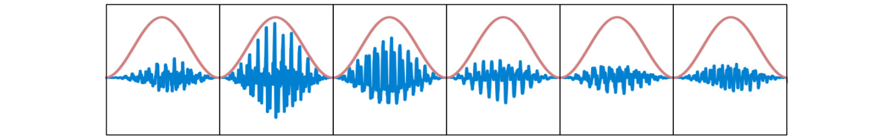
The discrete Fourier transform assumes that the input signal is periodic. In other words, the last sample of the 1024-element input buffer is expected to smoothly loop back to the first sample in that same buffer. That most likely won’t be the case for the kind of audio signals we’ll be working with!

If we were to loop the contents of the FIFO, there would be a discontinuity every time it jumped back to the beginning. This kind of discontinuity creates what’s known as spectral leakage. The frequency spectrum requires a lot of additional frequencies to capture the discontinuity, which makes the spectrum less clear to understand.

What we’d wish to see is a single peak at the sine wave’s frequency (around 530 Hz) but in the spectrum obtained from the FFT, the frequencies above and below are also used, with amplitudes up to –32 dB. That doesn’t mean the spectrum is incorrect — it isn’t — but those extra frequencies make it harder to analyze what’s going on.

To avoid this mess and get a spectrum that only has information we actually care about, we apply a windowing function to the input data before taking the FFT. This window tapers off the waveform near the start and end of the FFT frame, so that now it can loop without sudden jumps.

There are many different windowing functions but the one we’ll use is the Hann window, basically a modified cosine shape. The windowed input and its spectrum look like this:

The peak still isn’t super sharp (that would only happen if the sine frequency falls exactly on a bin boundary) but the other frequencies have been reduced a lot in magnitude and are no longer cluttering up the spectrum.

The window solves the issue of spectral leakage and gives a much cleaner spectrum, but now we have a new problem:

If we were to take the FFT of this windowed signal and immediately convert it back using the inverse FFT, in theory this should give us the original audio again, since we didn’t make any changes to the spectrum. In other words, the output from the IFFT should null with the input audio. Unfortunately, it doesn’t…

Since we apply the Hann window before taking the FFT, what we recover after the IFFT isn’t the original audio but the windowed version. Looking at these output FFT frames over time, we get a sequence that looks like this:

We need some way to remove the effect of the windowing from the output, since that up-and-down modulation of the amplitude will actually add a pitched tone to the audio.

The solution is to partially overlap the FFT frames. Each frame is still 1024 samples long, but if we use an overlap factor of 4 – also called 75% overlap – then we’ll perform the FFT after every 256 samples (known as the hopSize) instead of every 1024 samples.

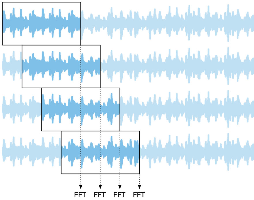
On the output side, we’ll also overlap the frames by adding them up. This process is known as overlap-add, and it’s how we construct the final output audio stream.

Usually before adding the frame to the output FIFO, we apply the window again. This is especially important if you change the spectrum’s phase information, as that can create discontinuities at the edges of the output frame, causing audio glitches during overlap-add.

For the overlap-add process to give the correct results it’s important that you choose an appropriate window shape and overlap amount. As mentioned, we’ll be using the Hann window, both before the FFT and after the IFFT, with an overlap of 75%. This works well because applying a window twice is the same as squaring it and a sequence of squared Hann windows nicely add up to a constant value where they overlap. (Note: the combined window does have a bit of gain, which we’ll correct for later.)

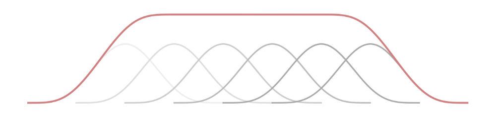
This is known as the COLA criterion, for constant overlap-add. However, not all window shapes and overlap amounts satisfy this criterion — for example, the Hann window with only 50% overlap will not work correctly (when used on both FFT and IFFT).

To recap: The FFTProcessor collects input samples into a FIFO of size 1024, but takes the FFT every 256 timesteps. It stores the results into the output FIFO by adding them to the existing contents of that FIFO.

OK enough theory, let’s look at some code!

The FFTProcessor class

Here is the public interface from FFTProcessor.h:

class FFTProcessor
{
public:
    FFTProcessor();
    int getLatencyInSamples() const;
    void reset();
    void processSample(float& sample, bool bypassed);
    void processBlock(float* data, int numSamples, bool bypassed);

private:
    ...
};

The main method is processSample(). This places the new sample into the input FIFO and performs the FFT processing every hopSize (= 256) samples. It also reads from the output FIFO and returns that value.

In the main PluginProcessor.h file, I added a member variable inside the AudioProcessor class’s private section:

private:
    FFTProcessor fft[2];

The FFTProcessor class is mono, so you need two instances to process stereo sound.

In PluginProcessor.cpp, in prepareToPlay(), we need to let the host know what the plug-in’s latency is and we also reset the FFTProcessor’s internal state. Recall that the output is always delayed by the length of the FFT frame, in our case 1024 samples.

void FFTExampleAudioProcessor::prepareToPlay(
    double sampleRate, int samplesPerBlock)
{
    setLatencySamples(fft[0].getLatencyInSamples());

    fft[0].reset();
    fft[1].reset();
}

To keep things simple for this example, the AudioProcessor only supports stereo sound:

bool FFTExampleAudioProcessor::isBusesLayoutSupported(const BusesLayout& layouts) const
{
    return layouts.getMainOutputChannelSet() == juce::AudioChannelSet::stereo();
}

The audio processing code looks as follows:

void FFTExampleAudioProcessor::processBlock(
    juce::AudioBuffer<float>& buffer, juce::MidiBuffer& midiMessages)
{
    juce::ScopedNoDenormals noDenormals;
    auto numInputChannels = getTotalNumInputChannels();
    auto numOutputChannels = getTotalNumOutputChannels();
    auto numSamples = buffer.getNumSamples();

    for (auto i = numInputChannels; i < numOutputChannels; ++i) {
        buffer.clear(i, 0, numSamples);
    }

    bool bypassed = apvts.getRawParameterValue("Bypass")->load();

    float* channelL = buffer.getWritePointer(0);
    float* channelR = buffer.getWritePointer(1);

    for (int sample = 0; sample < numSamples; ++sample) {
        float sampleL = channelL[sample];
        float sampleR = channelR[sample];

        sampleL = fft[0].processSample(sampleL, bypassed);
        sampleR = fft[1].processSample(sampleR, bypassed);

        channelL[sample] = sampleL;
        channelR[sample] = sampleR;
    }
}

This is a typical JUCE audio processing loop. It calls fft.processSample() on each sample and writes the result back into the AudioBuffer.

The plug-in has only one parameter, Bypass, that toggles the plug-in on or off. I added this so we can test that the FFT logic correctly handles being bypassed. The value of the bypass parameter is passed into fft.processSample().

By the way, it’s also possible to process the entire block at once. In that case you would write the following instead of the sample-by-sample loop. Which approach to use depends on how the rest of your plug-in is processing the audio. Internally, fft.processBlock() calls processSample() anyway.

    for (int channel = 0; channel < numInputChannels; ++channel) {
        auto* channelData = buffer.getWritePointer(channel);
        fft[channel].processBlock(channelData, numSamples, bypassed);
    }

The rest of PluginProcessor.cpp is pretty much all template code, so let’s move on to the fun stuff.

The variables

The FFTProcessor class defines a few constants that describe the size of the FFT frame and the amount of overlap.

static constexpr int fftOrder = 10;
static constexpr int fftSize = 1 << fftOrder;      // 1024 samples
static constexpr int numBins = fftSize / 2 + 1;    // 513 bins
static constexpr int overlap = 4;                  // 75% overlap
static constexpr int hopSize = fftSize / overlap;  // 256 samples

To make the FFT larger or smaller, change the fftOrder constant. It’s defined this way to guarantee the length in fftSize is always a power of two. The FFT outputs fftSize/2 + 1 frequency bins that describe the spectrum (the numBins variable). The hopSize is the overlap expressed in number of samples.

For this example project, we’re using the built-in JUCE FFT and WindowingFunction objects. These are member variables of FFTProcessor.

juce::dsp::FFT fft;
juce::dsp::WindowingFunction<float> window;

Since this uses juce::dsp objects, the project needs to include the juce_dsp module. JUCE’s built-in FFT is not necessarily the fastest around, so you might want to swap in another FFT library for better performance. That’s left as an exercise for the reader.

We also need some variables to manage the FIFOs:

int count = 0;
int pos = 0;
std::array<float, fftSize> inputFifo;
std::array<float, fftSize> outputFifo;

The pos variable keeps track of the current write position in the input FIFO as well as the output FIFO. Since both FIFOs have the same length, the position is always the same for both. The count variable counts up to 256 (the hopSize) so that we know when we need to take the FFT next. The FIFOs themselves are regular std::array objects.

Finally, we need an array that’s used to pass data to and from the juce::dsp::FFT object. This array will contain interleaved complex numbers, which is why the length is fftSize * 2, as each complex number is made up of two floats:

std::array<float, fftSize * 2> fftData;

FFTProcessor has a reset() method that zeros out everything:

void FFTProcessor::reset()
{
    count = 0;
    pos = 0;
    std::fill(inputFifo.begin(), inputFifo.end(), 0.0f);
    std::fill(outputFifo.begin(), outputFifo.end(), 0.0f);
}

This is the method we called from AudioProcessor’s prepareToPlay earlier. There’s no need to zero out the fftData array because we’ll always overwrite its contents before taking the FFT anyway.

Creating the window

In FFTProcessor.cpp, the FFTProcessor constructor looks like this:

FFTProcessor::FFTProcessor() :
    fft(fftOrder),
    window(fftSize + 1, juce::dsp::WindowingFunction<float>::WindowingMethod::hann, false)
{
}

The juce::dsp::FFT object is easy to initialize: it takes just one argument that describes the length of the FFT frame. Here fftOrder = 10, to make a 2^10 = 1024 element FFT.

The WindowingFunction object requires a bit more explanation. The window is just another array of length fftSize, and to apply the window to the signal we’ll multiply each sample in the FFT buffer with the corresponding sample from the window.

For convenience, we’re using JUCE’s WindowingFunction, but JUCE windows are symmetric, while we need the window to be periodic for the overlap-add process to work out correctly.

Symmetrical means the first and last values in the array are identical, while periodic means the last value smoothly leads back to the first value if we were to loop the contents of the array. In the symmetrical case, the partially overlapping windows do not sum to a constant everywhere they overlap. (Recall that the FFT assumes the input is periodic too.)

To work around this issue, I’m simply making the WindowingFunction one sample larger than it needs to be, fftSize + 1, but we’ll only use the first fftSize samples. Without this + 1, the overlap-add logic doesn’t properly null with the original audio — yep, that one sample makes a big difference.

JUCE’s WindowingFunction also has a normalise argument, which is true by default but we’re setting it to false. Since the edges taper off, the average value over the Hann window is not 1.0 but 0.5, meaning that we lose half the energy in the audio frame after multiplying it by the window. As a result, any peaks in the spectrum will be 6 dB lower than their true value.

We could compensate for this by setting normalise to true, which makes the window taller to give it an average value of 1.0. However, the overlap-add process introduces a gain of its own that we need to compensate for later, and the values I’m using for that compensation assume the Hann window is not normalized. Just a little gotcha to be aware of.

processSample

Let’s get to the star of the show, the processSample() method of FFTProcessor. It’s actually very simple:

float FFTProcessor::processSample(float sample, bool bypassed)
{
    inputFifo[pos] = sample;   // 1

    float outputSample = outputFifo[pos];  // 2
    outputFifo[pos] = 0.0f;

    pos += 1;
    if (pos == fftSize) {  // 3
        pos = 0;
    }

    count += 1;
    if (count == hopSize) {  // 4
        count = 0;
        processFrame(bypassed);
    }

    return outputSample;  // 5
}

How this works, step-by-step:

1. Push the new sample value into the input FIFO.

2. Read the output value from the output FIFO. Once we’ve read the sample value, set this position in the output FIFO back to zero so we can add new IFFT results to it later. This is necessary to clear out stale values that belong to samples that have already been played.

3. Advance the FIFO index and wrap around if necessary.

4. Process the FFT frame once we’ve collected hopSize new samples.

5. Return the sample we read from the output FIFO, so the host can play it.

Since the hop size is 256 samples, 255 out of 256 times this function just writes the current input value into the input FIFO and reads the delayed output value from the output FIFO, and immediately returns. But on the 256th timestep, it calls processFrame() to perform the FFT and the spectral processing.

processFrame

This is a private method in FFTProcessor where we do all the FFT, inverse transform, and overlap-add stuff. Let’s look at it piece-by-piece. First, we need to copy the contents of the input FIFO into the fftData array.

void FFTProcessor::processFrame(bool bypassed)
{
    const float* inputPtr = inputFifo.data();
    float* fftPtr = fftData.data();

    std::memcpy(fftPtr, inputPtr + pos, (fftSize - pos) * sizeof(float));
    if (pos > 0) {
        std::memcpy(fftPtr + fftSize - pos, inputPtr, pos * sizeof(float));
    }

Since the input FIFO is a circular buffer that wraps around when we get to the end, the current index (the pos variable) can be pointing anywhere inside the buffer when this function is called. In practice, since fftSize is an exact multiple of hopSize, pos will also be a multiple of hopSize when we get here, i.e. 0, 256, 512, or 768.

Because we incremented pos after writing to the input FIFO, it is one beyond the most recent sample that was written. In other words, the value under pos is the oldest one in the buffer and it will be overwritten on the next timestep. The value directly prior to pos is the newest one in the buffer (the one we just wrote).

The FFT input buffer in fftData needs to have the oldest sample in position 0 and the newest one in position 1023. So, we copy the FIFO in two parts into the FFT working space.

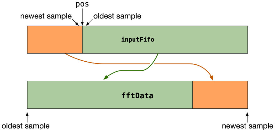
Note that fftData is actually fftSize * 2 elements long but here we only copy over the first fftSize elements. The remainder of the array remains uninitialized / filled with junk. This is fine as the juce::dsp::FFT object doesn’t read from that half, it will only need it as internal working space.

Next, we apply the window to avoid spectral leakage. That’s pretty easy with JUCE’s WindowingFunction. This uses SIMD under the hood so it’s fast.

    window.multiplyWithWindowingTable(fftPtr, fftSize);

Now that we’ve copied the input audio into the FFT buffer and applied the window, we can perform the FFTs:

    if (!bypassed) {
        fft.performRealOnlyForwardTransform(fftPtr, true);  // FFT
        processSpectrum(fftPtr, numBins);
        fft.performRealOnlyInverseTransform(fftPtr);        // IFFT
    }

Pretty straightforward! Here, fftPtr is a pointer to the contents from the fftData array. The forward transform reads audio data from this array and overwrites it with the spectrum, and the inverse transform does the opposite.

The second argument to performRealOnlyForwardTransform() tells the FFT object that it should only calculate half the spectrum — the positive frequencies only — as we don’t need the negative frequencies and it is faster.

processSpectrum() is where you’d do your actual spectral processing. We’ll look at this method in a minute.

Once the spectral stuff is done, we apply the window again:

    window.multiplyWithWindowingTable(fftPtr, fftSize);

    for (int i = 0; i < fftSize; ++i) {
        fftPtr[i] *= windowCorrection;
    }

The first window was to avoid spectral leakage from possible discontinuities at the edges of the incoming FFT frame. The second window serves the same purpose but for the outgoing frame. It’s possible to skip this second window, but this may give glitches in the audio from the overlap-add operation, in particular when your spectral processing modifies the phase.

In addition, we apply a gain correction. The value for this is defined in FFTProcessor.h:

static constexpr float windowCorrection = 2.0f / 3.0f;

When using a Hann window twice, with 75% overlap, the resulting amplitude is 1.5× too large. Recall that the average value of the Hann window is 0.5. Applying a window twice means we’re effectively multiplying by the square of the window, and the squared Hann window has an average value of 0.375 or 3/8. Due to the overlap factor, the total gain is 4 × 3/8 = 1.5. To compensate we should divide by this value, which is equivalent to multiplying by 2/3. For other windows and other overlap factors, this correction will be different.

Finally, we can add the contents of fftData to the output FIFO. Just like the input FIFO, we need to do this in two parts because the current write index may be located anywhere in the circular buffer. I’ve implemented this with a simple for-loop, but this could be optimized using JUCE’s FloatVectorOperations class.

    for (int i = 0; i < pos; ++i) {
        outputFifo[i] += fftData[i + fftSize - pos];
    }
    for (int i = 0; i < fftSize - pos; ++i) {
        outputFifo[i + pos] += fftData[i];
    }
}

Phew, that concludes all the plumbing we need in order to do FFT processing in a plug-in! The remaining part is processSpectrum(), which is where you’ll actually analyze and modify the frequency spectrum. But first a few words about how to interpret the spectrum data.

The spectrum is complex

We used fft.performRealOnlyForwardTransform() to perform the FFT. The term real-only means that the input data consists of real-valued numbers, in this case audio samples.

There is also fft.perform() which assumes the input buffer is filled with values of type std::complex<float>. You could certainly use this version, with the real part of the complex number set to the sample value and the imaginary part set to zero, but it’s slower and ultimately gives the same results. You’d also have to deal with the negative frequencies explicitly, while you can safely ignore those when using the real-only FFT (this treats the negative frequencies as the complex conjugates of the positive frequencies).

performRealOnlyForwardTransform() reads the audio samples from the fftData array and overwrites them with complex numbers that represent the frequency information. Even though the type of fftData is std::array<float>, after taking the FFT it contains complex numbers. These are interleaved, so if you were to print out the contents of fftData, you’d get real, imaginary, real, imaginary, ... and so on.

That’s why fftData has length fftSize * 2, because for every floating-point number from the waveform domain we get two floats in the frequency domain.

However… only the first (fftSize/2 + 1) complex numbers contain valid frequency information. For convenience, I defined this value in the numBins variable. The reason of course, is that in digital audio we can only use frequencies up to Nyquist (half the sampling rate). The other elements in fftData are used internally by the juce::dsp::FFT object, and weird stuff happens when you overwrite them, so you shouldn’t touch those.

In other words, for our 1024-element FFT, the spectrum is described by 513 complex numbers that represent the frequency bins. Each of these bins covers a bandwidth of sampleRate / 1024 = 48000 / 1024 = 46.875 Hz. The first bin is for the DC offset (0 Hz), the last bin is at the Nyquist limit.

When doing the inverse Fourier transform, fft.performRealOnlyInverseTransform() also only looks at the first fftSize/2 + 1 bins. Afterwards, the first 1024 floating-point numbers of fftData contain audio data again (and the rest is junk).

processSpectrum

The final method we haven’t implemented yet is processSpectrum(). This is where you do whatever it is you want to do:

void FFTProcessor::processSpectrum(float* data, int numBins)
{
    auto* cdata = reinterpret_cast<std::complex<float>*>(data);

    for (int i = 0; i < numBins; ++i) {
        float magnitude = std::abs(cdata[i]);
        float phase = std::arg(cdata[i]);

        // This is where you'd do your spectral processing...

        cdata[i] = std::polar(magnitude, phase);
    }
}

Since fftData now contains complex numbers instead of plain floats, I find it more useful to cast this to array<std::complex> so we can work directly with the complex number type.

You almost never access the real and imaginary parts of the complex number directly. Instead, you’d convert these to a magnitude and phase value using std::abs() and std::angle(), respectively, and work with those values.

The spectral processing code in processSpectrum() loops through the frequency bins. It calculates the magnitude and phase for each bin, does something interesting with them, and finally converts the new magnitude and phase values back to a complex number.

The example app has a silly example where we change the phase of each frequency bin somewhat randomly:

phase *= float(i);

but I’m sure you can come up with much more interesting effects!

Note that you don’t need to use a loop like I’ve shown here, you can do whatever you want in processSpectrum(), as long as you fill up the first numBins elements of the data array with complex numbers that represent the spectrum you want to output.

A note about FFT scaling

Some things to keep in mind:

• The forward FFT in JUCE produces magnitudes that are fftSize times “too large”. In other words, a 0 dB sine wave would show up in the spectrum as having a much louder amplitude of +60 dB or 20*log10(1024). When doing the IFFT, JUCE automatically divides by fftSize to bring everything back to the correct scale. This is a convention; other FFT libraries may do this scaling differently or give you a choice.

• Actually, the sine wave’s magnitude will appear to be 6 dB lower, because each frequency appears twice in the spectrum: once as a positive frequency and once as a negative frequency, and the energy is divided between them. When these two frequencies are combined again by the IFFT, that –6 dB factor disappears because multiplying by 2 is the same as boosting by 6 dB.

• In addition, because we use the Hann window before the FFT, which has an average value of 0.5, that makes everything another 6 dB (or 0.5×) smaller.

What this means for the spectral processing is that you may want to scale the magnitude values by 4/fftSize, if knowing the true decibel value is important to you. Just remember that the JUCE IFFT always divides the magnitudes by fftsize again when it converts the spectrum back to audio.

Using a null test to make sure

It’s a good idea to test that the logic works correctly before doing any spectral processing yet. To do this, comment out everything in processSpectrum() so that this method doesn’t modify the spectrum anymore.

We now have an FFT processor that goes through all the stages of the Short Time Fourier Transform but doesn’t alter the spectrum in any way. In theory, this should recover the original audio without changes, albeit with 1024 samples of latency. We can verify whether this is indeed the case using a null test.

In your DAW, create two tracks with the same sound clip and identical settings for volume and panning. Put an instance of the plug-in on the second track. Also set this track to invert the phase. In some DAWs, such as Logic Pro, you’ll need to use a separate Gain plug-in for this.

Since both tracks output the same audio, inverting the phase on the second track causes its output to be subtracted from the first track’s output and what remains — if the FFT plug-in properly nulls — is silence. To check that, put a spectrum analyzer such as Voxengo SPAN on the output or master bus. This should show absolutely nothing happening.

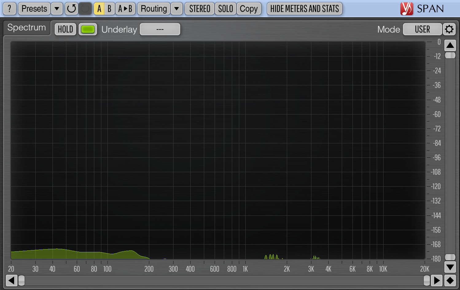
If you set the vertical scale of the spectrum analyzer to –180 dB, you might still see some activity at the very bottom. This is due to floating point precision limitations. 32-bit floats have 24 bits of precision, which corresponds to –144 dB. Since it’s possible to see signal below that, the FFT processing logic isn’t entirely lossless, but the difference is so tiny that it doesn’t matter.

Also try toggling the plug-in’s Bypass parameter to verify that this works. You shouldn’t hear any difference with bypass enabled or disabled and the audio should null in both cases. (Note that the bypass parameter may not be hooked up to your DAW’s own bypass button. For this test it’s best to use the Bypass parameter from the plug-in UI.)

Great, I’d say that properly nulls! It’s always a good idea to do this check, so that you can be sure the overlap-add logic and choice of window are correct. If the FFT processing doesn’t null, chances are you’re using the wrong window for the chosen overlap factor or hop size, or the gain correction or FFT scaling factor is incorrect.

Using your own window

Let’s say you wanted to use a window that’s not supported by JUCE’s WindowingFunction, such as the Vorbis window. You can easily define it yourself.

In the class definition in FFTProcessor.h you would replace the WindowingFunction variable with a simple array:

std::array<float, fftSize> window;

Note that now the length is fftSize, not fftSize + 1, since we can guarantee the window is periodic.

Just for the sake of demonstration I’m going to implement the same Hann window we’ve been using all along, so you can see that it’s pretty straightforward. You can find formulas for other windowing functions on Wikipedia.

static void hannWindow(float* window, int length)
{
    float delta = 6.28318500518798828125f / float(length);
    float phase = 0.0f;
    for (int i = 0; i < length; ++i) {
        window[i] = 0.5f * (1.0f - std::cos(phase));
        phase += delta;
    }
}

And then in the constructor you’d call it as follows:

hannWindow(window.data(), windowSize);

In processFrame(), you can apply the window as follows:

    for (int i = 0; i < fftSize; ++i) {
        fftPtr[i] *= window[i];
    }

Instead of having a loop you could use juce::FloatVectorOperations::multiply to take advantage of SIMD. Optimizing this is left as an exercise for the reader.

The end

There are many possible variations of this FFT processing loop, but hopefully this gives you a good starting point to build your own.

To summarize, the steps we performed were:

1. collect enough samples to fill up the FFT input buffer
2. apply a window to remove discontinuities at the edges
3. perform the forward FFT to get the spectrum
4. do spectral processing on the frequency bins using complex numbers
5. perform the inverse FFT to convert the spectrum back to audio
6. apply the window again
7. output the processed samples using overlap-add

Let me know if you have any questions!