Krunch Saturator

Some time ago I came across the 1 Euro Filter, an adaptive filter designed to balance jitter and lag in noisy input for interactive systems. I was curious what it would sound like when applied to audio. Pretty good actually! The filter adds harmonics in an interesting way. So I turned it into a free plug-in named Krunch.

In this blog post I will talk a bit about how the 1 Euro Filter works and why it sounds like a saturation effect when used to process audio.

You can grab the code and VST3/AU files from GitHub.

How to use Krunch

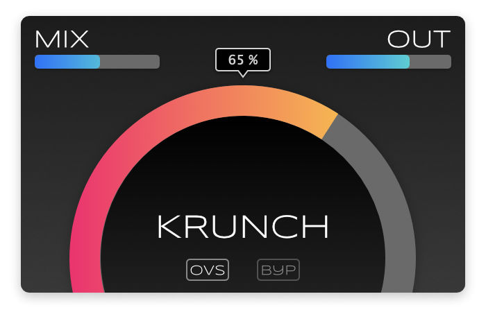
Krunch combines low-pass filtering with saturation. It has the following controls:

• KRUNCH The higher this is dialed up, the more the sound will be filtered. But even at low values it will already add crunch.

• MIX The effect works best when some dry signal is mixed in. For example, set KRUNCH to 75% and MIX to 50% to make kicks stand out more.

• OUT Since this is a filter, the output signal may end up being a tad quieter. Compensate the drop in loudness with this slider.

• OVS Enable oversampling. Gives a cleaner result because fewer aliases, but aliases have a charm of their own so you may want to leave this disabled.

• BYP Bypass the plug-in for A/B testing.

Suggested workflow: Set MIX to 100%, dial KRUNCH to where it sounds nasty, then reduce MIX again to bring some of the high end back. Toggle BYP to compare and bring up OUT to equalize the loudness. Adding just a bit of subtle saturation is usually enough!

What is the 1 Euro Filter?

The 1 Euro Filter was originally published in the paper 1€ Filter: A Simple Speed-based Low-pass Filter for Noisy Input in Interactive Systems by Géry Casiez, Nicolas Roussel and Daniel Vogel (2012).

The goal of the 1 Euro Filter is to remove noise — high frequency components — from the input signal. This noise is also known as jitter. Applying a low-pass filter gets rid of the jitter but also introduces lag that reduces responsiveness, which is problematic in systems that rely on interactive feedback.

The solution is to use an adaptive low-pass filter where the filter’s cutoff frequency is dynamically computed using the rate of change of the input signal.

• When the signal is changing slowly, the cutoff frequency can be low to remove as much noise as possible. The lag is now higher but matters less. For slow movements, it’s more important to remove the jitter than the lag.

• As the speed of the movement increases, the filter’s cutoff is automatically raised to reduce lag. This lets more noise through, but for responding to fast movements it’s more important to remove the lag than the jitter.

The filter itself is just a basic one-pole filter:

y[n] = alpha * x[n] + (1 - alpha) * y[n - 1]

Or how I personally like to write it:

y[n] += alpha * (x[n] - y[n - 1])

When the cutoff frequency for the filter is low, the filter coefficient alpha is a small number. Since we do alpha * x[n], new sample values are slow to be incorporated into the filter’s output y[n], which is what creates the lag. To reduce the lag, the cutoff frequency must be raised, which lets more noise through. So there’s a trade-off here.

The filter coefficient alpha is calculated using the following formula:

r = 2π * cutoff
alpha = r / (r + sampleRate)

Here, cutoff is the cutoff frequency of the filter in Hz. What makes the 1 Euro Filter an adaptive filter is that cutoff isn’t a fixed value but changes based on the input signal. In other words, the filter’s cutoff point is being modulated by the input, as opposed to a more typical modulation source such as an LFO or envelope.

I’m not sure why they chose this particular coefficient calculation. It’s different from the usual alpha = 1 - exp(-2π * frequency / sampleRate) that is often used with one-pole filters. Granted, the authors of the paper didn’t have audio in mind and they were not trying to replicate the transfer function of an analog RC circuit.

It doesn’t really matter that the coefficient formula is different than usual — it simply won’t give the kind of frequency response you might be used to at higher frequencies. At 1 kHz, the –3 dB point is where it should be, but at 2 kHz it’s already shifted a bit. For a cutoff of 20 kHz, the –3 dB point is around 11k.

One advantage of this coefficient formula is that it allows the cutoff value to go over Nyquist — something that will actually happen a lot — without blowing up the filter. If cutoff is at Nyquist, alpha becomes 0.758546993 or exactly π/(π + 1), regardless of the sample rate. In fact, alpha asymptotically approaches 1.0 but never exceeds it, no matter how large cutoff becomes. So the filter is always stable.

Computing the cutoff frequency

Now the question is, where does cutoff come from? Unlike a regular filter, the 1 Euro Filter’s cutoff frequency is computed dynamically, it’s not set to a predetermined value.

In the paper they use the discrete derivative of the signal, which is simply:

derivative = (x[n] - y[n - 1]) / T

where T is the time in seconds between these two samples. In the case of digital audio, the samples are uniformly spaced in time and T = 1/sampleRate, so we can write this as:

derivative = (x[n] - y[n - 1]) * sampleRate

The derivative of a signal gives us the rate of change or the “speed” of the movement. If two successive samples are similar, the derivative is small because there isn’t much change from one sample to the next. This is what happens at low frequencies. The more dissimilar the two samples are, the larger the rate of change, and the higher the signal’s frequency.

The derivative is smoothed using another one-pole filter with its own coefficient, dalpha:

derivative_smoothed += dalpha * (derivative - derivative_smoothed)

Smoothing the derivative removes short bursts of noise that aren’t part of a true faster signal. This smoothing happens slowly because the dalpha coefficient is very small. It’s computed using the same coefficient formula shown earlier but with a fixed cutoff of 1 Hz. That makes dalpha equal to 2π/(2π + sampleRate), which is 0.00013 at 48 kHz.

At any instant, the value of derivative can be quite large but derivative_smoothed is slow to catch up. Through experimentation I found this was essential to making the algorithm work well. Although keep in mind that we’re processing 48000 samples per second, so slow is a relative concept.

Finally, the adaptive cutoff frequency is calculated using a simple linear equation:

cutoff = min_cutoff + beta * abs(derivative_smoothed)

Here, min_cutoff and beta are two tweakable parameters that let you tune the filter. As the paper’s website says, “If high speed lag is a problem, increase beta. If slow speed jitter is a problem, decrease min_cutoff.”

What this formula means: If the derivative is larger, the rate of change is faster, and so the cutoff frequency is shifted upwards. The beta parameter is there to amplify this effect — the larger beta is, even small changes in the signal will have a large result. So, for a large beta you can expect less filtering to happen and more high frequencies to be let through.

By the way, the derivative can be positive or negative, so the abs() makes the direction of the change unimportant. We only care about its magnitude.

The code

Clearly the 1 Euro Filter wasn’t designed for sound. However, that shouldn’t stop us from applying this filter to audio signals! By tuning the algorithm we might get something that hopefully sounds good… or at least interesting.

Krunch is a fairly typical JUCE plug-in. Most of the code is for handling the user interface but I’ll skip discussing that. The filter itself is implemented in the class OneEuroFilter.

Let’s go over the interesting parts, starting with the function that does the actual filtering:

double operator()(double x) noexcept
{
    // 1
    double dx = (x - z) * 40000.0;

    // 2
    dy += dalpha * (dx - dy);

    // 3
    double cutoff = 1.0 + beta * std::abs(dy);

    // 4
    double alpha = smoothingFactor(cutoff);
    y += alpha * (x - y);
    z += alpha * (y - z);

    // 5
    return z;
}

Step-by-step this is what it does:

1. Calculate the derivative dx. The input sample is x. The output sample from the previous timestep is in the variable z. Instead of multiplying with the sample rate as in the paper, this uses the constant 40000.0 instead.

2. Smoothen the derivative and put it into dy. This is a regular one-pole filter with coefficient dalpha. As mentioned, this coefficient is very small and so dy only changes slowly.

3. Calculate the adaptive cutoff frequency. This uses the absolute value of the smoothened derivative dy from the previous step. beta is derived from the setting of the KRUNCH knob. I’ve fixed min_cutoff to 1.0.

4. Filter the input signal using the new cutoff. Since a one-pole filter only has a 6 dB/octave slope, I put two of these filters in series.

5. Output the filtered sample value.

The function smoothingFactor calculates the filter coefficient:

double smoothingFactor(double cutoff) const noexcept
{
    double r = 6.28318530717958647692528676655900577 * cutoff;
    return r / (r + sampleRate);
}

Finally, setKrunch configures the amount of krunchiness by setting the beta variable:

void setKrunch(double krunch) noexcept
{
    const double kk = krunch * krunch;
    double skewed = kk * kk;
    beta = 1.0 + 20000.0 * skewed;
}

This is hooked up to the plug-in parameter for the KRUNCH knob. When the knob is turned off, krunch is 1.0, and when the knob is fully dialed in, krunch is 0.0. First this skews the parameter value, making it easier to dial in low frequencies. beta is then a value between 1 and 20000 Hz.

In the paper they’re not filtering audio but readings from inexpensive controllers such as a Kinect or Wiimote, with sampling rates of around 100 Hz. The values for min_cutoff and beta they use make no sense for our digital audio signals.

After some experimentation I decided to use the value 40000.0 in the derivative calculation rather than the sample rate. Using a constant makes the filter independent of the sampling rate, which allows for oversampling. The sampling rate is only used to calculate the filter coefficients alpha and dalpha. Together with a maximum value of 20000.0 for beta this sounds quite nice.

Intuition for how it works

If you load Krunch into Plugindoctor or another EQ analyzer, it plots the following frequency response:

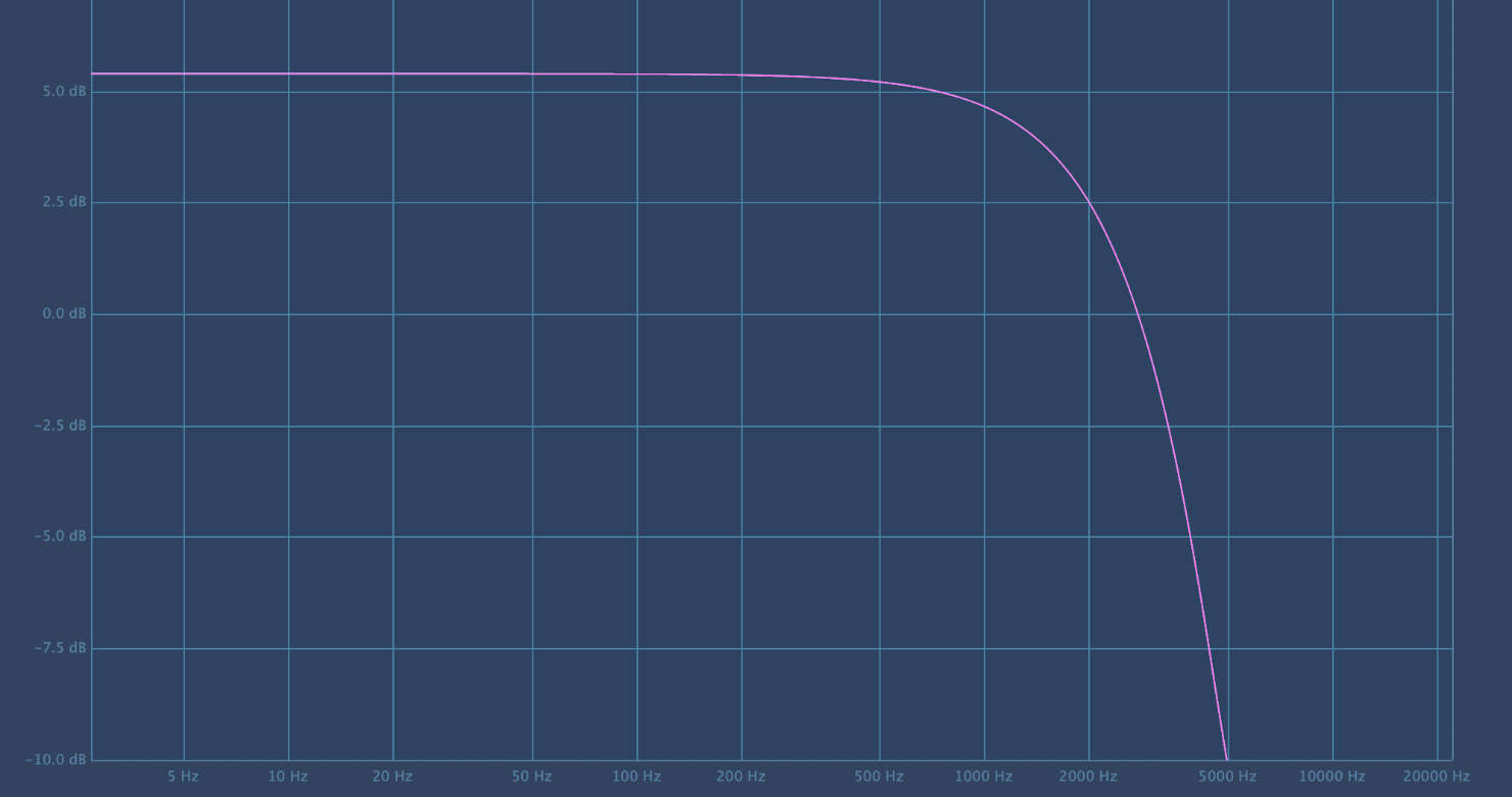
That is indeed a low-pass filter. However, the gain is a bit weird: a one-pole filter should not boost the gain. This happens because the filter is not time-invariant — after all, the filter cutoff is modified on every sample timestep — and a frequency response such as calculated by Plugindoctor is only meaningful for LTI systems. (See also this excellent Dan Worrall video.)

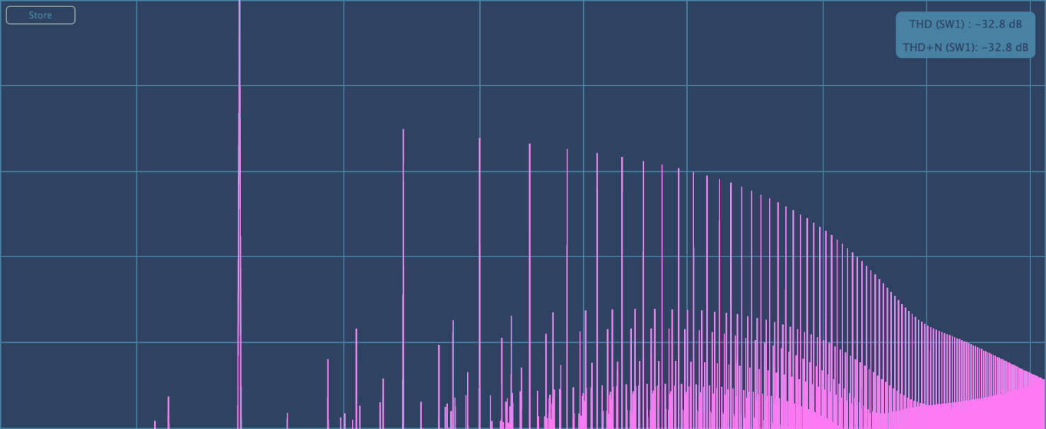
Plugindoctor’s HarmonicAnalysis mode indeed shows plenty of odd harmonics. There are also aliases, which is why the plug-in also has an 8× oversampling mode.

When the KRUNCH dial is at 0%, beta will be 20000 and so the cutoff frequency will be around Nyquist and no filtering happens. As you push KRUNCH up, beta becomes smaller, causing cutoff to drop, filtering more and more high end out of the signal.

What creates the saturation effect is the modulation of the cutoff frequency. Let’s say you have a clean sine wave. Filtering this with a low-pass makes the amplitude of the sine wave lower, assuming the cutoff is somewhere below the sine’s frequency.

Modulating the cutoff then makes the amplitude of the sine wave go up and down. Since this happens very rapily, the resulting signal no longer looks like a clean sine wave but a distorted one. Hence, harmonics have been introduced and it sounds like a saturation effect.

Of course, since this is still a low-pass filter, you lose some of the high end. That’s why the plug-in has a dry/wet mix control as well, to bring some of that high end back in.

Give Krunch a go and let me know how you like the sound!